Montbrio SDE model using Cupy
Estimation of global coupling \(G\).
![]()
[34]:
import os
import vbi
import torch
import numpy as np
import networkx as nx
from copy import deepcopy
import sbi.utils as utils
import matplotlib.pyplot as plt
from sbi.analysis import pairplot
from vbi.inference import Inference
from vbi.models.cupy.mpr import MPR_sde

import warnings
warnings.filterwarnings("ignore")
[2]:
seed = 42
np.random.seed(seed)
[3]:
LABESSIZE = 10
plt.rcParams['axes.labelsize'] = LABESSIZE
plt.rcParams['xtick.labelsize'] = LABESSIZE
plt.rcParams['ytick.labelsize'] = LABESSIZE
loading connectivity matrix
[4]:
D = vbi.LoadSample(nn=88)
weights = D.get_weights()
nn = weights.shape[0]
print(f"number of nodes: {nn}")
number of nodes: 88
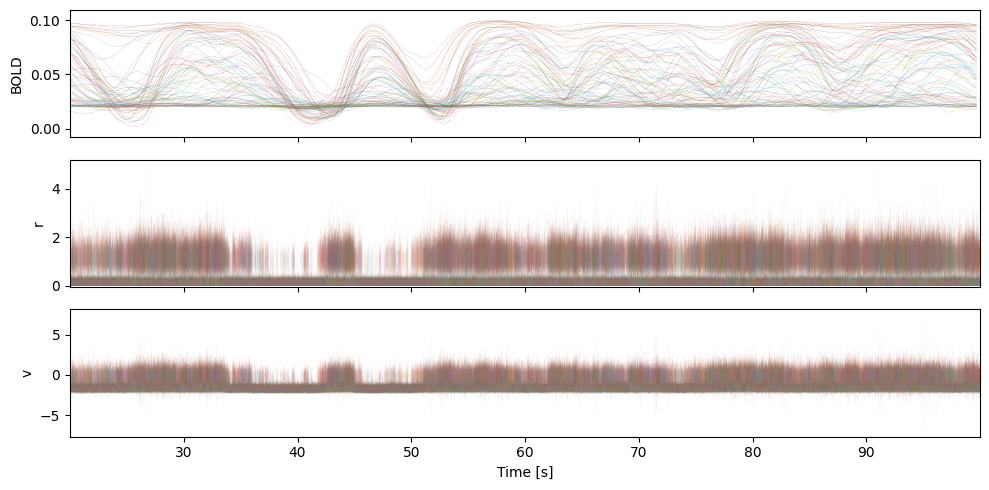
Simulating BOLD single for a sample value of \(G\)
[5]:
TR = 300.0
fs = 1 / (TR / 1000)
t_cut = 20
par = {
    "G": 0.506,  # global coupling strength
    "weights": weights,  # connection matrix
    "method": "heun",  # integration method
    "dt": 0.01,
    "t_cut": 20_000,
    "t_end": 100_000,  # [ms]
    "num_sim": 1,  # number of simulations
    "tr": TR,
    "rv_decimate": 10,
    "engine": "cpu",  # cpu or gpu
    "seed": seed,  # seed for random number generator
    "RECORD_RV": True,
    "RECORD_BOLD": True,
}
[6]:
obj = MPR_sde(par)
# print(obj())
sol = obj.run()
Integrating: 100%|██████████| 999999/999999 [02:50<00:00, 5876.29it/s]
[9]:
rv_d = sol["rv_d"]
rv_t = sol["rv_t"] / 1000
fmri_d = sol["fmri_d"]
fmri_t = sol["fmri_t"] / 1000

rv_d = rv_d
rv_t = rv_t
fmri_d = fmri_d
fmri_t = fmri_t
print(np.isnan(fmri_d).sum(), np.isnan(rv_d).sum())

print(f"rv_t.shape = {rv_t.shape}")
print(f"rv_d.shape = {rv_d.shape}")
print(f"fmri_d.shape = {fmri_d.shape}")
print(f"fmri_t.shape = {fmri_t.shape}")

np.savez(
    "bold_obs.npz", t=fmri_t, bold=np.transpose(fmri_d, (2, 1, 0)), theta=par["G"]
)
0 0
rv_t.shape = (79999,)
rv_d.shape = (79999, 176, 1)
fmri_d.shape = (266, 88, 1)
fmri_t.shape = (266,)
[10]:
if fmri_d.ndim == 3:
    fig, ax = plt.subplots(3, figsize=(10, 5), sharex=True)
    ax[0].set_ylabel("BOLD")
    ax[0].plot(fmri_t, fmri_d[:,:,0], lw=0.1)
    ax[0].margins(0, 0.1)
    ax[1].plot(rv_t, rv_d[:, :nn, 0], lw=0.1, alpha=0.1)
    ax[2].plot(rv_t, rv_d[:, nn:, 0], lw=0.1, alpha=0.1)
    ax[1].set_ylabel("r")
    ax[2].set_ylabel("v")
    ax[2].set_xlabel("Time [s]")
    ax[1].margins(0, 0.01)
    plt.tight_layout()
    plt.show()
Training data
Uniform prior for \(G\) and sampling from prior;
Selecting GPU as engine;
Storing training BOLD signals;
Extracting features from the simulated BOLD signals;
Visualizing some of the features;
Training NN and estimating parameter of G for given observed signal;
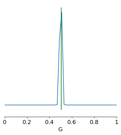
Visualising the posterior distribution.
[26]:
num_sim = 512
G_min, G_max = 0.0, 1.0

prior_min = [G_min]
prior_max = [G_max]
prior = utils.torchutils.BoxUniform(
    low=torch.as_tensor(prior_min), high=torch.as_tensor(prior_max)
)

obj = Inference()
theta = obj.sample_prior(prior, num_sim, seed=seed)

par1 = deepcopy(par)
par1['G'] = theta.numpy().astype(np.float64).squeeze()
par1['num_sim'] = num_sim
par1['engine'] = 'gpu'
par1['RECORD_RV'] = False
[ ]:
obj = MPR_sde(par)
sol = obj.run()
[15]:
fmri_d = sol["fmri_d"]
fmri_t = sol["fmri_t"]
fmri_d = fmri_d
fmri_t = fmri_t
bolds = np.transpose(fmri_d, (2, 1, 0))

os.makedirs("output", exist_ok=True)
np.savez("output/bolds.npz", bolds=bolds, fmri_t=fmri_t, theta=theta.numpy().squeeze())
print(f"fmri_d.shape = {fmri_d.shape}")
print(f"fmri_t.shape = {fmri_t.shape}")
fmri_d.shape = (332, 88, 512)
fmri_t.shape = (332,)
[17]:
bolds = np.load("output/bolds.npz")["bolds"]
theta = np.load("output/bolds.npz")["theta"]
theta = torch.tensor(theta).float()
[40]:
from vbi import (
    get_features_by_domain,
    get_features_by_given_names,
    report_cfg,
    extract_features,
)

cfg = get_features_by_domain("connectivity")
cfg = get_features_by_given_names(cfg, ["fcd_stat"])
report_cfg(cfg)
Selected features:
------------------
■ Domain: connectivity
 ▢ Function:  fcd_stat
   ▫ description:  Extracts features from dynamic functional connectivity (FCD)
   ▫ function   :  vbi.feature_extraction.features.fcd_stat
   ▫ parameters :  {'TR': 1.0, 'win_len': 30, 'positive': False, 'eigenvalues': True, 'masks': None, 'verbose': False, 'pca_num_components': 3, 'quantiles': [0.05, 0.25, 0.5, 0.75, 0.95], 'features': ['sum', 'max', 'min', 'mean', 'std', 'skew', 'kurtosis']}
   ▫ tag        :  ['fmri', 'eeg', 'meg']
   ▫ use        :  yes
[50]:
df = extract_features(bolds, fs, cfg, n_workers=10, output_type="dataframe")
df = df[["fcd_full_sum", "fcd_full_ut_std"]]
df['G'] = theta.numpy().squeeze()
df.to_csv("output/g_cupy_features.csv", index=False)
df.head()
100%|██████████| 512/512 [00:07<00:00, 68.90it/s]
[50]:
| fcd_full_sum | fcd_full_ut_std | G | |
|---|---|---|---|
| 0 | 9478.422852 | 0.031059 | 0.429404 |
| 1 | NaN | NaN | 0.885443 |
| 2 | 9770.584961 | 0.032312 | 0.573904 |
| 3 | 9611.076172 | 0.033598 | 0.266580 |
| 4 | 9417.106445 | 0.027417 | 0.627449 |
[51]:
df.columns
[51]:
Index(['fcd_full_sum', 'fcd_full_ut_std', 'G'], dtype='object')
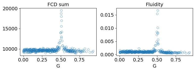
[52]:
LABELSIZE = 14
plt.rc('axes', labelsize=LABELSIZE)
plt.rc('axes', titlesize=LABELSIZE)
plt.rc('figure', titlesize=LABELSIZE)
plt.rc('legend', fontsize=LABELSIZE)
plt.rc('xtick', labelsize=LABELSIZE)
plt.rc('ytick', labelsize=LABELSIZE)

f_kwargs = {
    "lw": 1,
    "alpha": 0.5,
    "marker": "o",
    "linestyle": "",
    "markerfacecolor": "none",
}

fig, ax = plt.subplots(1,2, figsize=(8, 3))
ax[0].plot(df["G"], df["fcd_full_sum"], **f_kwargs)
ax[1].plot(df["G"], df["fcd_full_ut_std"]**2, **f_kwargs)

titles = ["FCD sum", "Fluidity"]
for i in range(2):
    ax[i].set_xlabel("G")
    ax[i].set_title(titles[i])
plt.tight_layout()
[53]:
# drop G column
X = df.drop(columns=["G"]).values
X = torch.tensor(X, dtype=torch.float32)
[54]:
obj_inf = Inference()
posterior = obj_inf.train(theta, X, prior=prior, num_threads=4)
WARNING:root:Found 132 NaN simulations and 0 Inf simulations. They will be excluded from training.
Neural network successfully converged after 367 epochs.train Done in 0 hours 0 minutes 06.877320 seconds
Observation point
[55]:
bold_obs = np.load("bold_obs.npz")['bold']
x_obs = extract_features(bold_obs, 0.3, cfg, output_type="dataframe")
x_obs = x_obs[["fcd_full_sum", "fcd_full_ut_std"]].values
samples = obj_inf.sample_posterior(x_obs, 10000, posterior)

limits = [[i, j] for i, j in zip(prior_min, prior_max)]
fig, ax = pairplot(
    samples,
    points=[par['G']],
    figsize=(5, 5),
    limits=limits,
    labels=["G"],
    diag="kde",
    fig_kwargs=dict(
        points_offdiag=dict(marker="*", markersize=10),
        points_colors=["g"],
    ),
)
100%|██████████| 1/1 [00:00<00:00, 7.22it/s]
[ ]: