Jansen-Rit whole brain (NUMBA)
[1]:
import os
import vbi
import torch
import pickle
import numpy as np
from tqdm import tqdm
import networkx as nx
import sbi.utils as utils
import matplotlib.pyplot as plt
from multiprocessing import Pool
from sbi.analysis import pairplot
from vbi.sbi_inference import Inference
from vbi.models.numba.jansen_rit import JR_sde
from sklearn.preprocessing import StandardScaler
[2]:
from vbi import report_cfg, update_cfg
from vbi import extract_features_df
from vbi import get_features_by_domain, get_features_by_given_names
from helpers import *
[3]:
seed = 2
np.random.seed(seed)
torch.manual_seed(seed);
path = "output/jr_numba/"
os.makedirs(path, exist_ok=True)
[4]:
LABESSIZE = 12
plt.rcParams['axes.labelsize'] = LABESSIZE
plt.rcParams['xtick.labelsize'] = LABESSIZE
plt.rcParams['ytick.labelsize'] = LABESSIZE
[5]:
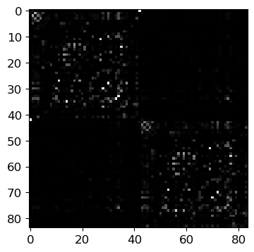
D = vbi.LoadSample(nn=84)
weights = D.get_weights()
nn = weights.shape[0]
print(f"number of nodes: {nn}")

fig, ax = plt.subplots(1, 1, figsize=(4, 4.5))
ax.imshow(weights, cmap="gray", vmin=0, vmax=1);
number of nodes: 84
[6]:
par = {
    "G": 1.0,
    "mu": 0.24,
    "noise_amp": 0.1,
    "dt": 0.05,
    "C0": 135.0 * 1.0,
    "C1": 135.0 * 0.8,
    "C2": 135.0 * 0.25,
    "C3": 135.0 * 0.25,
    "weights": weights,
    "t_cut": 500.0,      # ms
    "t_end": 2501.0,     # ms
    "seed": seed,
    "decimate": 1
}
[7]:
jr = JR_sde(par)
print(jr)
==============================================================================================================
JR_sde
==============================================================================================================

Model Parameters:
--------------------------------------------------------------------------------------------------------------
Parameter       | Description                              | Value/Shape                    | Type
--------------------------------------------------------------------------------------------------------------
A               | Excitatory EPSP amplitude                | 3.25                           | scalar
B               | Inhibitory IPSP amplitude                | 22.0                           | scalar
C0              | Synapses: pyramidal to excitatory        | shape (84,)                    | vector
C1              | Synapses: excitatory to pyramidal        | shape (84,)                    | vector
C2              | Synapses: pyramidal to inhibitory        | shape (84,)                    | vector
C3              | Synapses: inhibitory to pyramidal        | shape (84,)                    | vector
G               | Global coupling strength                 | 1.0                            | scalar
a               | Inverse time constant of EPSP            | 0.1                            | scalar
b               | Inverse time constant of IPSP            | 0.05                           | scalar
decimate        | Decimation factor for output             | 1                              | int
dt              | Integration time step                    | 0.05                           | scalar
initial_state   | Initial state vector (6*nn)              | shape (504,)                   | vector
mu              | Mean external input                      | 0.24                           | scalar
noise_amp       | Noise amplitude                          | 0.1                            | scalar
r               | Slope of sigmoid at v0                   | 0.56                           | scalar
seed            | Random seed for reproducibility          | 2                              | int
t_cut           | Cut-off time for output                  | 500.0                          | scalar
t_end           | End time of simulation                   | 2501.0                         | scalar
v0              | Potential at half max firing rate        | 6.0                            | scalar
vmax            | Maximum firing rate                      | 0.005                          | scalar
weights         | Structural connectivity matrix           | shape (84, 84)                 | matrix
==============================================================================================================
[8]:
# G, C1
theta_true = [1.5, 135]
[9]:
# C1 needs to be a vector of size nn
C1 = theta_true[1]
theta_true_dict = {"G": 1.0, "C1":C1}
data = jr.run(theta_true_dict)

print(data['t'].shape, data['x'].shape)
(40020,) (40020, 84)
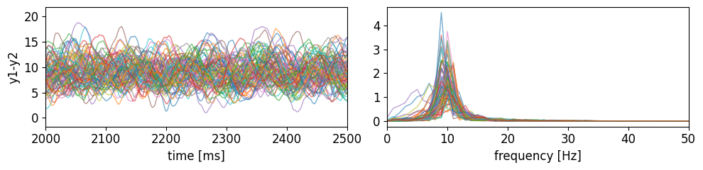
[10]:
fig, ax = plt.subplots(1, 2, figsize=(10, 2.5))
plot_ts_pxx_jr({"t": data['t'], "x": data['x'].T}, par, [ax[0], ax[1]], alpha=0.6, lw=1)
ax[0].set_xlim(2000, 2500)
plt.tight_layout()
[11]:
cfg = get_features_by_domain(domain="spectral")
cfg = get_features_by_given_names(cfg, names=['spectrum_stats', 'spectrum_auc', "spectrum_moments"])
update_cfg(cfg, "spectrum_stats", {"fs": 1000/ par['dt'], "method": "welch", "average":True})
update_cfg(cfg, "spectrum_auc", {"fs": 1000/ par['dt'], "method": "welch", "average":True})
update_cfg(cfg, "spectrum_moments", {"fs": 1000/ par['dt'], "method": "welch", "average":True})
report_cfg(cfg)
Selected features:
------------------
■ Domain: spectral
 ▢ Function:  spectrum_stats
   ▫ description:  Computes the spectrum of the signal.
   ▫ function   :  vbi.feature_extraction.features.spectrum_stats
   ▫ parameters :  {'fs': 20000.0, 'nperseg': None, 'indices': None, 'verbose': False, 'average': True, 'method': 'welch', 'features': ['spectral_distance', 'fundamental_frequency', 'max_frequency', 'max_psd', 'median_frequency', 'spectral_centroid', 'spectral_kurtosis', 'spectral_variation']}
   ▫ tag        :  all
   ▫ use        :  yes
 ▢ Function:  spectrum_moments
   ▫ description:  Computes the spectrum of the signal.
   ▫ function   :  vbi.feature_extraction.features.spectrum_moments
   ▫ parameters :  {'fs': 20000.0, 'nperseg': None, 'method': 'welch', 'moments': [2, 3, 4, 5, 6], 'normalize': False, 'verbose': False, 'indices': None, 'average': True}
   ▫ tag        :  all
   ▫ use        :  yes
 ▢ Function:  spectrum_auc
   ▫ description:  Computes the area under the curve of the signal computed with trapezoid rule.
   ▫ function   :  vbi.feature_extraction.features.spectrum_auc
   ▫ parameters :  {'fs': 20000.0, 'nperseg': None, 'method': 'welch', 'average': True, 'verbose': False, 'bands': [[0, 4], [4, 8], [8, 12], [12, 30], [30, 70]], 'indices': None}
   ▫ tag        :  all
   ▫ use        :  yes
[12]:
from copy import deepcopy

def wrapper(par, control, cfg, verbose=False, with_labels=False):
    g, c1 = control
    par1 = deepcopy(par)
    control = {"G": g, "C1": c1}

    ode = JR_sde(par1)
    sol = ode.run(control)

    # extract features
    fs = 1.0 / par['dt'] * 1000  # [Hz]
    stat = extract_features_df(ts=[sol['x'].T],
                                      cfg=cfg,
                                      fs=fs,
                                      n_workers=1,
                                      verbose=verbose)
    value = stat.values
    if with_labels:
        label = list(stat.columns)
        return value[0], label
    return value[0]
[13]:
def batch_run(par, control_list, cfg, n_workers=1):
    n = len(control_list)
    def update_bar(_):
        pbar.update()
    with Pool(processes=n_workers) as pool:
        with tqdm(total=n) as pbar:
            async_results = [pool.apply_async(wrapper,
                                              args=(
                                                  par, control_list[i], cfg, False),
                                              callback=update_bar)
                             for i in range(n)]
            stat_vec = [res.get() for res in async_results]
    return stat_vec
[14]:
x_, labels = wrapper(par, theta_true, cfg, with_labels=True)
len(x_), labels
[14]:
(18,
 ['spectral_distance_0',
  'fundamental_frequency_0',
  'max_frequency_0',
  'max_psd_0',
  'median_frequency_0',
  'spectral_centroid_0',
  'spectral_kurtosis_0',
  'spectral_variation_0',
  'spectrum_moment_2',
  'spectrum_moment_3',
  'spectrum_moment_4',
  'spectrum_moment_5',
  'spectrum_moment_6',
  'spectrum_auc_0',
  'spectrum_auc_1',
  'spectrum_auc_2',
  'spectrum_auc_3',
  'spectrum_auc_4'])
[15]:
num_sim = 1000
num_workers = 10
C1_min, C1_max = 130.0, 300.0
G_min, G_max = 0.0, 5.0
prior_min = [G_min, C1_min]
prior_max = [G_max, C1_max]
prior = utils.BoxUniform(low=torch.tensor(prior_min),
                         high=torch.tensor(prior_max))
[16]:
obj = Inference()
theta = obj.sample_prior(prior, num_sim) # sample from prior with uniform distribution
theta_np = theta.numpy().astype(float)
produce training data
[ ]:
stat_vec = batch_run(par, theta_np, cfg, num_workers)
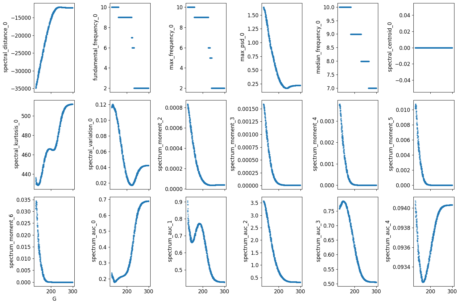
Visualizing the feature distribution vs global coupling/C1
[18]:
stat_vec_arr = np.array(stat_vec)
fig, axes = plt.subplots(3, 6, figsize=(15, 10), sharex=True)
for i in range(stat_vec_arr.shape[1]):
    axes[i // 6, i % 6].scatter(theta_np[:, 1], stat_vec_arr[:, i], s=5, alpha=0.5)
    axes[i // 6, i % 6].set_ylabel(f" {labels[i]}")
axes[-1, 0].set_xlabel("G")
plt.tight_layout()
# turn off axis for empty subplots
for ax in axes.flat:
    if not ax.has_data():
        ax.axis('off')
standardizing the features (optional)
droping features with small variance
[19]:
import os
os.makedirs('output', exist_ok=True)

scaler = StandardScaler()
stat_vec_st = scaler.fit_transform(np.array(stat_vec))
# drop columns with zero variance, keep indices of remaining columns
non_zero_var_indices = np.var(stat_vec_st, axis=0) > 1e-6
stat_vec_st = stat_vec_st[:, non_zero_var_indices]
stat_vec_st = torch.tensor(stat_vec_st, dtype=torch.float32)

torch.save(theta, path + 'theta.pt')
torch.save(stat_vec_st, path + 'stat_vec.pt')
print(theta.shape, stat_vec_st.shape)
torch.Size([1000, 2]) torch.Size([1000, 17])
[ ]:
posterior = obj.train(theta, stat_vec_st, prior, method="SNPE", density_estimator="maf")
[21]:
xo = wrapper(par, theta_true, cfg)
xo_st = scaler.transform(xo.reshape(1, -1))
xo_st = xo_st[:, non_zero_var_indices]
[22]:
samples = obj.sample_posterior(xo_st, 10000, posterior)
torch.save(samples, path + 'samples.pt')
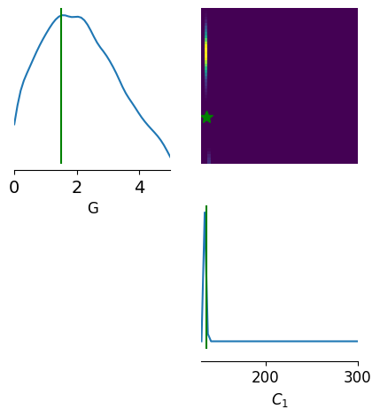
[23]:
limits = [[i, j] for i, j in zip(prior_min, prior_max)]
points = [theta_true]
fig, ax = pairplot(
    samples,
    limits=limits,
    figsize=(5, 5),
    points=points,
    labels=["G", r"$C_{1}$"],
    upper="kde",
    diag="kde",
    fig_kwargs=dict(
        points_offdiag=dict(marker="*", markersize=10),
        points_colors=["g"],
    ),
)
ax[0, 0].tick_params(labelsize=14)
ax[0, 0].margins(y=0)
fig.savefig(path + "jr_sde_cpp.jpeg", dpi=300)
[ ]: