# Number of brain regions/nodes
nn = 4
# Create a simple connectivity matrix (undirected, symmetric)
# Adjust connection strengths to control coupling
weights = np.array(
[
[0.0, 0.15, 0.05, 0.0],
[0.15, 0.0, 0.15, 0.05],
[0.05, 0.15, 0.0, 0.15],
[0.0, 0.05, 0.15, 0.0],
]
)
# Inter-regional distances (tr_len) can be:
# Option 1: Scalar - applied uniformly to all connected pairs
# tr_len = 10.0
#
# Option 2: Matrix (nn, nn) - specific distances for each pair
tr_len = np.array([
[0.0, 10.0, 8.0, 0.0],
[10.0, 0.0, 12.0, 9.0],
[8.0, 12.0, 0.0, 11.0],
[0.0, 9.0, 11.0, 0.0],
])
# Option 3: No delays
# tr_len = np.zeros_like(weights) # No delays for simplicity
par = {
"nn": nn,
"weights": weights,
"a": 0.20, # Bifurcation parameter: 0.15-0.30 for oscillations
"omega": 2.0
* np.pi
* 0.040, # Angular frequency (rad/ms) = 2*pi*f_Hz/1000, here 40 Hz
"G": 0.6, # Coupling strength: 0.0 (uncoupled) to 1.0 (strong)
"sigma": 0.01, # Noise amplitude: 0.0 (deterministic) to 0.1 (noisy)
"dt": 0.01, # Timestep (ms): MUST be small (~0.01) for stability at high frequencies
"t_end": 300.0, # Total simulation time (ms)
"t_cut": 100.0, # Transient cutoff (ms): discard initial transients
"speed": 5.0, # Conduction velocity (mm/ms)
"tr_len": tr_len, # Typical inter-regional distance (mm)
"seed": 42, # Random seed: change for different realizations
"RECORD_X": True, # Record complex neural activity
"x_decimate": 10, # Decimation factor for X recording
}
# ============================================================================
# 2. Initialize and run simulation
# ============================================================================
print("Initializing Stuart-Landau model...")
model = SL_sde(par=par)
print(model)
print("Warming up ...")
tic = time.time()
result = model.run()
print(f"Warmup Simulation finished in {time.time()-tic:.2f} seconds.")
tic = time.time()
result = model.run()
print(f"Simulation finished in {time.time()-tic:.2f} seconds.")
# Extract results
t = result["t"]
X = result["X"] # Complex neural activity: shape (time, nn)
print(f"Simulation completed!")
print(f" Time points recorded: {len(t)}")
print(f" Number of regions: {X.shape[1]}")
# ============================================================================
# 3. Analyze and visualize results
# ============================================================================
# Compute amplitude and phase from complex activity
amplitude = np.abs(X) # Magnitude of oscillation
phase = np.angle(X) # Phase of oscillation
print(f"\nActivity statistics:")
for i in range(nn):
print(
f" Region {i}: amplitude mean={amplitude[:, i].mean():.4f}, "
f"std={amplitude[:, i].std():.4f}"
)
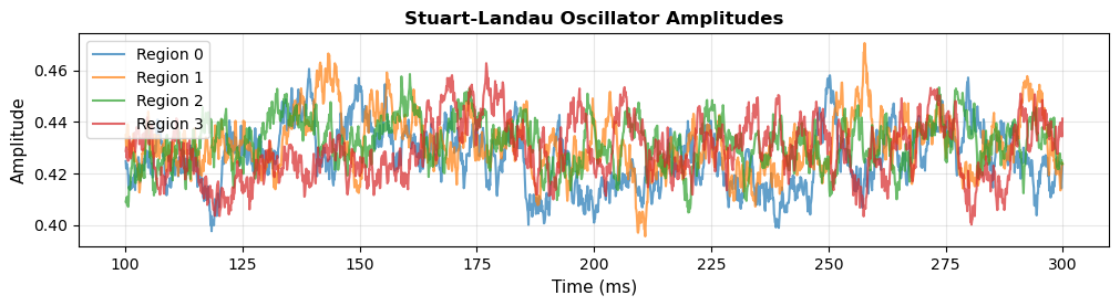
# Create visualization
fig, ax = plt.subplots(1, figsize=(12, 2.5))
# Plot 1: Amplitude over time
for i in range(nn):
ax.plot(t, amplitude[:, i], label=f"Region {i}", alpha=0.7, linewidth=1.5)
ax.set_xlabel("Time (ms)", fontsize=11)
ax.set_ylabel("Amplitude", fontsize=11)
ax.set_title("Stuart-Landau Oscillator Amplitudes", fontsize=12, fontweight="bold")
ax.legend(loc="best")
ax.grid(True, alpha=0.3)
plt.show()