Jansen-Rit whole brain (NUMBA)

# Install VBI package in Google Colab (lightweight, CPU-only version)
print("Setting up VBI for Google Colab...")

# Skip C++ compilation for faster installation in Colab
%env SKIP_CPP=1

print("Environment configured.")

# Install the package
# !pip install vbi

print("VBI package installed successfully! Ready to proceed.")

1. Imports & Global Configuration

import os
from copy import deepcopy
from multiprocessing import Pool

import numpy as np
import autograd.numpy as anp
import matplotlib.pyplot as plt
from tqdm import tqdm
from scipy import signal
from sklearn.preprocessing import StandardScaler

import vbi
from vbi.models.numba.jansen_rit import JR_sde
from vbi import report_cfg, update_cfg
from vbi import extract_features_df
from vbi import get_features_by_domain, get_features_by_given_names
from vbi.utils import BoxUniform, posterior_shrinkage_numpy, posterior_zscore_numpy
from vbi.cde import MAFEstimator  # your (sbi-like) CDE estimator

def plot_ts_pxx_jr(data, par, ax, **kwargs):
    tspan = data['t']
    y = data['x']
    ax[0].plot(tspan, y.T, label='y1 - y2', **kwargs)
    freq, pxx = signal.welch(y, 1000/par['dt'], nperseg=y.shape[1]//2)
    ax[1].plot(freq, pxx.T, **kwargs)
    ax[1].set_xlim(0, 50)
    ax[1].set_xlabel("frequency [Hz]")
    ax[0].set_xlabel("time [ms]")
    ax[0].set_ylabel("y1-y2")
    ax[0].margins(x=0)

    plt.tight_layout()

Reproducibility & output

RNG_SEED: int = 2
np.random.seed(RNG_SEED)

OUT_DIR = "output/jansen_rit_sde_numba_cde_/"
os.makedirs(OUT_DIR, exist_ok=True)

Matplotlib aesthetics

LABEL_SIZE = 12
plt.rcParams["axes.labelsize"] = LABEL_SIZE
plt.rcParams["xtick.labelsize"] = LABEL_SIZE
plt.rcParams["ytick.labelsize"] = LABEL_SIZE

Data/control flags

LOAD_DATA: bool = True   # <— Set True to load cached dataset if available
SAVE_DATA: bool = True   # Save dataset after (re)simulation
CACHE_FILE = os.path.join(OUT_DIR, "jr_cde_dataset.npz")

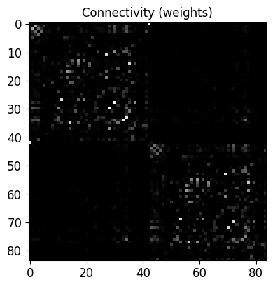
2. Structural Connectivity & Preview

Load sample connectome (nn: number of nodes) and preview

sample = vbi.LoadSample(nn=84)
CONNECTIVITY = sample.get_weights()
N_NODES = CONNECTIVITY.shape[0]
print(f"number of nodes: {N_NODES}")

number of nodes: 84

Quick visual check of the adjacency (can be toggled off if desired)

if True:
    fig, ax = plt.subplots(1, 1, figsize=(4, 4.5))
    im = ax.imshow(CONNECTIVITY, cmap="gray", vmin=0, vmax=1)
    ax.set_title("Connectivity (weights)")
    plt.tight_layout()

3. Simulator parameters & one reference run

JR SDE base parameters (units: ms where applicable)

SIM_CFG = {
    "G": 1.0,            # global coupling (will be overridden per-control)
    "mu": 0.24,          # external input
    "noise_amp": 0.1,
    "dt": 0.05,          # ms
    "C0": 135.0 * 1.0,
    "C1": 135.0 * 0.8,
    "C2": 135.0 * 0.25,
    "C3": 135.0 * 0.25,
    "weights": CONNECTIVITY,
    "t_cut": 500.0,      # ms — discard transient
    "t_end": 2501.0,     # ms — total duration
    "seed": RNG_SEED,
    "decimate": 1,
}

Reference ground truth parameters for evaluation/plots

TRUE_THETA = np.array([1.5, 135.0], dtype=np.float32)  # [G, C1]
TRUE_CONTROL = {"G": float(TRUE_THETA[0]), "C1": float(TRUE_THETA[1])}

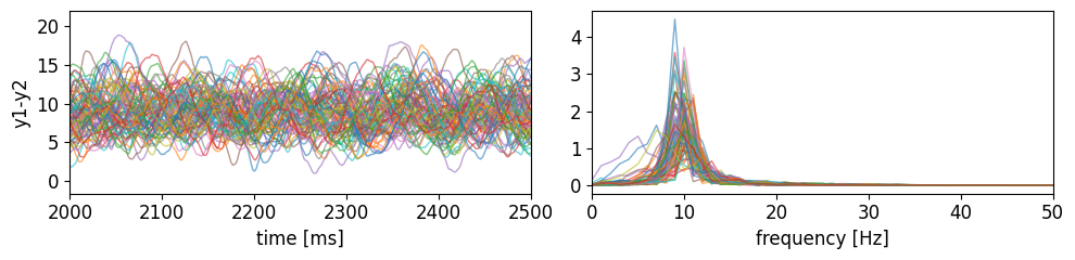
One quick simulation preview

jr_ref = JR_sde(SIM_CFG)
ref_sol = jr_ref.run(TRUE_CONTROL)
print(ref_sol["t"].shape, ref_sol["x"].shape)

(40020,) (40020, 84)

Time series + spectrum preview

fig, ax = plt.subplots(1, 2, figsize=(10, 2.5))
plot_ts_pxx_jr({"t": ref_sol["t"], "x": ref_sol["x"].T}, SIM_CFG, [ax[0], ax[1]], alpha=0.6, lw=1)
ax[0].set_xlim(2000, 2500)
plt.tight_layout()

4. Feature configuration (spectral domain)

Configure spectral features and fix sampling frequency

feat_cfg = get_features_by_domain(domain="spectral")
feat_cfg = get_features_by_given_names(
    feat_cfg, names=["spectrum_stats", "spectrum_auc", "spectrum_moments"]
)
fs_hz = 1000.0 / SIM_CFG["dt"]  # Hz
for key in ("spectrum_stats", "spectrum_auc", "spectrum_moments"):
    update_cfg(feat_cfg, key, {"fs": fs_hz, "method": "welch", "average": True})
report_cfg(feat_cfg)

Selected features:
------------------
■ Domain: spectral
 ▢ Function:  spectrum_stats
   ▫ description:  Computes the spectrum of the signal.
   ▫ function   :  vbi.feature_extraction.features.spectrum_stats
   ▫ parameters :  {'fs': 20000.0, 'nperseg': None, 'indices': None, 'verbose': False, 'average': True, 'method': 'welch', 'features': ['spectral_distance', 'fundamental_frequency', 'max_frequency', 'max_psd', 'median_frequency', 'spectral_centroid', 'spectral_kurtosis', 'spectral_variation']}
   ▫ tag        :  all
   ▫ use        :  yes
 ▢ Function:  spectrum_moments
   ▫ description:  Computes the spectrum of the signal.
   ▫ function   :  vbi.feature_extraction.features.spectrum_moments
   ▫ parameters :  {'fs': 20000.0, 'nperseg': None, 'method': 'welch', 'moments': [2, 3, 4, 5, 6], 'normalize': False, 'verbose': False, 'indices': None, 'average': True}
   ▫ tag        :  all
   ▫ use        :  yes
 ▢ Function:  spectrum_auc
   ▫ description:  Computes the area under the curve of the signal computed with trapezoid rule.
   ▫ function   :  vbi.feature_extraction.features.spectrum_auc
   ▫ parameters :  {'fs': 20000.0, 'nperseg': None, 'method': 'welch', 'average': True, 'verbose': False, 'bands': [[0, 4], [4, 8], [8, 12], [12, 30], [30, 70]], 'indices': None}
   ▫ tag        :  all
   ▫ use        :  yes

5. Simulation → feature pipeline (single & batch)

def simulate_and_extract(sim_cfg: dict, control_pair, cfg, *, return_labels=False, verbose=False):
    """Run JR SDE for control (G, C1) and extract features.
    Parameters
    ----------
    sim_cfg : dict
        Base simulator configuration (copied internally).
    control_pair : tuple(float, float)
        (G, C1) values.
    cfg : Any
        Feature-extraction configuration from vbi.
    return_labels : bool
        Also return the feature labels.
    Returns
    -------
    np.ndarray or (np.ndarray, list[str])
        Feature vector (and labels if requested).
    """
    g_val, c1_val = control_pair
    local_cfg = deepcopy(sim_cfg)
    controls = {"G": float(g_val), "C1": float(c1_val)}
    solver = JR_sde(local_cfg)
    sol = solver.run(controls)

    # Extract features per node, then aggregate as configured
    stats = extract_features_df(
        ts=[sol["x"].T], cfg=cfg, fs=fs_hz, n_workers=1, verbose=verbose
    )
    vec = stats.values[0]
    if return_labels:
        return vec, list(stats.columns)
    return vec

def run_batch(sim_cfg: dict, control_list, cfg, n_workers: int = 1):
    """Parallel batch of simulate_and_extract with a tqdm progress bar."""
    n_total = len(control_list)
    def _update(_):
        pbar.update()
    with Pool(processes=n_workers) as pool:
        with tqdm(total=n_total, desc="Simulations") as pbar:
            async_results = [
                pool.apply_async(
                    simulate_and_extract, args=(sim_cfg, control_list[i], cfg), callback=_update
                )
                for i in range(n_total)
            ]
            features_list = [res.get() for res in async_results]
    return features_list

Probe labels once

feat_vec_probe, FEATURE_LABELS = simulate_and_extract(SIM_CFG, TRUE_THETA, feat_cfg, return_labels=True)
print(f"n_features (raw): {len(feat_vec_probe)}")

n_features (raw): 18

6. Prior and sampling of parameters (θ)

Define box prior for [G, C1]

G_MIN, G_MAX = 0.0, 5.0
C1_MIN, C1_MAX = 130.0, 300.0
PRIOR_BOUNDS_MIN = [G_MIN, C1_MIN]
PRIOR_BOUNDS_MAX = [G_MAX, C1_MAX]
PRIOR = BoxUniform(low=PRIOR_BOUNDS_MIN, high=PRIOR_BOUNDS_MAX)

Simulation campaign settings

N_SIMULATIONS: int = 200
N_WORKERS: int = 10

7. Dataset build (with LOAD_DATA control)

if LOAD_DATA and os.path.exists(CACHE_FILE):
    # Reuse previously generated features and parameters
    cache = np.load(CACHE_FILE, allow_pickle=True)
    THETA = cache["theta"].astype(np.float32)
    FEATURES = cache["features"].astype(np.float32)
    SCALER_MEAN = cache["scaler_mean"].astype(np.float32)
    SCALER_SCALE = cache["scaler_scale"].astype(np.float32)
    NONZERO_MASK = cache["nonzero_mask"].astype(bool)
    FEATURE_LABELS = list(cache["labels"].tolist())
    print(f"Loaded cached dataset: {FEATURES.shape} features for {THETA.shape[0]} samples")
else:
    # Fresh simulations
    THETA = PRIOR.sample(N_SIMULATIONS, seed=RNG_SEED).astype(np.float32)
    raw_features = run_batch(SIM_CFG, THETA, feat_cfg, n_workers=N_WORKERS)
    FEATURES = np.asarray(raw_features, dtype=np.float32)

    # Standardize and optionally drop near-constant features
    scaler = StandardScaler()
    FEATURES = scaler.fit_transform(FEATURES).astype(np.float32)
    NONZERO_MASK = (np.var(FEATURES, axis=0) > 1e-6)
    FEATURES = FEATURES[:, NONZERO_MASK]
    SCALER_MEAN = scaler.mean_.astype(np.float32)
    # sklearn stores var_, convert to std as used in transform (avoid recomputing)
    SCALER_SCALE = scaler.scale_.astype(np.float32)
    if SAVE_DATA:
        np.savez(
            CACHE_FILE,
            theta=THETA,
            features=FEATURES,
            scaler_mean=SCALER_MEAN,
            scaler_scale=SCALER_SCALE,
            nonzero_mask=NONZERO_MASK,
            labels=np.array(FEATURE_LABELS, dtype=object),
        )
        print(f"Saved dataset cache → {CACHE_FILE}")

Simulations: 100%|██████████| 200/200 [01:09<00:00,  2.90it/s]

Saved dataset cache → output/jansen_rit_sde_numba_cde_/jr_cde_dataset.npz

8. Observation features (x₀) at TRUE_THETA

x0_vec = simulate_and_extract(SIM_CFG, TRUE_THETA, feat_cfg)
# Apply the same standardization/masking as training features
x0_std = ((x0_vec - SCALER_MEAN) / (SCALER_SCALE + 1e-12)).astype(np.float32)
x0_std = x0_std[NONZERO_MASK][None, :]  # shape (1, n_features_kept)

9. Train CDE (MAF) and sample posterior

NOTE: you can tune these (see your sbi-like MAF estimator)

maf_rng = anp.random.RandomState(RNG_SEED)
maf = MAFEstimator(n_flows=4, hidden_units=64)

Train on full (θ, x) pairs

maf.train(
    params=THETA,           # θ ∈ R^{N×2}
    features=FEATURES,      # x ∈ R^{N×M}
    n_iter=500,
    learning_rate=2e-4,
    use_tqdm=True,
)

Inferred dimensions: param_dim=2, feature_dim=17

Training: 100%|██████████| 500/500 [00:08<00:00, 57.77it/s, patience=3/20, train=-0.8013, val=-0.1472]

Draw posterior samples at x₀

posterior_samples = maf.sample(x0_std, n_samples=5000, rng=maf_rng)[0]

Diagnostics

shrinkage = posterior_shrinkage_numpy(THETA, posterior_samples)
zscores = posterior_zscore_numpy(TRUE_THETA, posterior_samples)
print("True parameters:      ", TRUE_THETA)
print("MAF mean estimate:    ", np.mean(posterior_samples, axis=0))
print("Posterior shrinkage:  ", np.array2string(shrinkage, precision=3, separator=", "))
print("Posterior z-score:    ", np.array2string(zscores, precision=3, separator=", "))

True parameters:       [  1.5 135. ]
MAF mean estimate:     [  2.0583837 134.67921  ]
Posterior shrinkage:   [-0.918,  0.999]
Posterior z-score:     [0.283, 0.185]

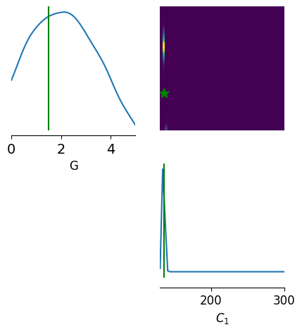
10. Visualization: posterior pairplot

from vbi.plot import pairplot_numpy

limits = [[lo, hi] for lo, hi in zip(PRIOR_BOUNDS_MIN, PRIOR_BOUNDS_MAX)]
point = TRUE_THETA.reshape(1, -1)
fig, ax = pairplot_numpy(
    posterior_samples,
    limits=limits,
    figsize=(5, 5),
    points=point,
    labels=["G", r"$C_{1}$"],
    upper="kde",
    diag="kde",
    fig_kwargs=dict(
        points_offdiag=dict(marker="*", markersize=10),
        points_colors=["g"],
    ),
)
ax[0, 0].tick_params(labelsize=14)
ax[0, 0].margins(y=0)
fig.savefig(os.path.join(OUT_DIR, "jr_sde_cde_pairplot.jpeg"), dpi=300)
print("Saved figure →", os.path.join(OUT_DIR, "jr_sde_cde_pairplot.jpeg"))

Saved figure → output/jansen_rit_sde_numba_cde_/jr_sde_cde_pairplot.jpeg