Wilson-Cowan SDE model in Numba

• sweep and inference with MAF

# Install VBI package in Google Colab (lightweight, CPU-only version)
print("Setting up VBI for Google Colab...")

# Skip C++ compilation for faster installation in Colab
%env SKIP_CPP=1

print("Environment configured.")

# Install the package
# !pip install vbi

print("VBI package installed successfully! Ready to proceed.")

Imports & global config

import os
import warnings
warnings.filterwarnings("ignore")

import numpy as np
import matplotlib.pyplot as plt
import multiprocessing as mp
from copy import deepcopy
from scipy.signal import welch

import vbi
from vbi.cde import MAFEstimator
from vbi.models.numba.wilson_cowan import WC_sde

Reproducibility and paths

GLOBAL_SEED = 42
np.random.seed(GLOBAL_SEED)

OUTPUT_DIR = "output/wilson_cowan_sde_numba_cde_"
os.makedirs(OUTPUT_DIR, exist_ok=True)

Matplotlib font sizes

LABEL_SIZE = 10
plt.rcParams["axes.labelsize"] = LABEL_SIZE
plt.rcParams["xtick.labelsize"] = LABEL_SIZE
plt.rcParams["ytick.labelsize"] = LABEL_SIZE

Frequency control tips (for reference) To shift oscillation frequency:

1. Coupling strengths (weights) 2) Time constants

2. External inputs 4) Refractory periods

3. Sigmoid parameters

Sweep over external input P (2-node toy network)

N_SWEEP = 30
P_grid = np.linspace(0.0, 3.0, N_SWEEP)

W_conn = np.array([[0, 1],
                   [1, 0]], dtype=np.float32)

params = dict(
    weights=W_conn,
    dt=0.1,
    t_end=2000.0,
    t_cut=101.0,
    noise_amp=0.001,
    g_e=0.0,
    g_i=0.0,
    P=1.22,
    RECORD_EI="EI",
    decimate=1,
    seed=GLOBAL_SEED,
)

def run_wc_with_P(params_dict: dict, P_value: float):
    """Run Wilson–Cowan SDE once with a specific external drive P."""
    sim = WC_sde(params_dict)
    sol = sim.run({"P": P_value})
    return sol

Parallel sweep

with mp.Pool(processes=4) as pool:
    sweep_results = pool.starmap(run_wc_with_P, [(params, p) for p in P_grid])
    sweep_results = [sol for sol in sweep_results if sol is not None]

t = sweep_results[0]["t"]
E_traces = np.array([sol["E"] for sol in sweep_results])
I_traces = np.array([sol["I"] for sol in sweep_results])

print(t.shape, E_traces.shape, I_traces.shape)  # (ntime,) (nsim, ntime, nnodes) (nsim, ntime, nnodes)

(18990,) (30, 18990, 2) (30, 18990, 2)

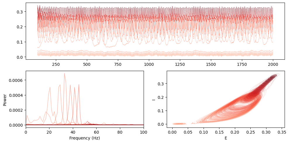
Visualize sweep: time series, spectra, and phase portrait

Welch PSD across sweep for node 0

freq, psd_E = welch(
    E_traces[:, :, 0],
    fs=1 / (params["dt"] * params["decimate"]) * 1000,
    nperseg=8 * 1024,
    axis=1,
)

mosaic = """
AA
BC
"""
fig = plt.figure(constrained_layout=True, figsize=(10, 5))
axs = fig.subplot_mosaic(mosaic)

colors = plt.cm.Reds(np.linspace(0.1, 1.0, N_SWEEP))

# Time series (E, node 0)
for i in range(N_SWEEP):
    axs["A"].plot(t, E_traces[i, :, 0], alpha=0.5, lw=0.5, color=colors[i])

# Spectra (E, node 0)
for i in range(N_SWEEP):
    axs["B"].plot(freq, psd_E[i, :], alpha=0.5, lw=1, color=colors[i], label=f"{P_grid[i]:.2f}")

# Phase portrait (E vs I, node 0)
for i in range(N_SWEEP):
    axs["C"].plot(E_traces[i, :, 0], I_traces[i, :, 0], lw=0.1, alpha=0.5, color=colors[i])

axs["B"].set_xlabel("Frequency (Hz)")
axs["B"].set_ylabel("Power")
axs["B"].set_xlim(0, 100)
axs["C"].set_xlabel("E")
axs["C"].set_ylabel("I")
plt.tight_layout()

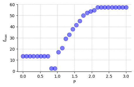
Peak frequency vs P

peak_idx = np.argmax(psd_E, axis=1)
f_peak = freq[peak_idx]

fig, ax = plt.subplots(figsize=(5, 3))
ax.plot(P_grid, f_peak, "bo", ms=10, alpha=0.5)
ax.grid(True, ls="--", lw=0.5)
ax.set_xlabel("P")
ax.set_ylabel(r"$f_{\max}$")
ax.spines["top"].set_visible(False)
ax.spines["right"].set_visible(False)

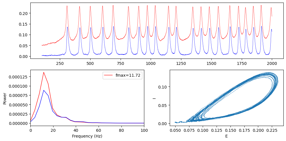
Single run (cleaner visualization)

W_conn = np.array([[0, 1],
                   [1, 0]], dtype=np.float32)
P0 = 1.025

params_single = {
    "g_e": 0.0,
    "seed": 42,
    "dt": 0.05,
    "t_end": 2000.0,
    "t_cut": 101.0,
    "noise_amp": 0.0005,  # small noise
    "decimate": 1,
    "P": P0,
    "RECORD_EI": "EI",
    "weights": W_conn,
}

sim_single = WC_sde(params_single)
sol_single = sim_single.run()
t1 = sol_single["t"]
E1 = sol_single["E"]
I1 = sol_single["I"]

print(t1.shape, E1.shape, I1.shape)

(37980,) (37980, 2) (37980, 2)

fE, psd_E1 = welch(
    E1,
    fs=1 / (params_single["dt"] * params_single["decimate"]) * 1000,
    nperseg=5 * 1024,
    axis=0,
)
fI, psd_I1 = welch(
    I1,
    fs=1 / (params_single["dt"] * params_single["decimate"]) * 1000,
    nperseg=5 * 1024,
    axis=0,
)

mosaic = """
AA
BC
"""
fig = plt.figure(constrained_layout=True, figsize=(10, 5))
axs = fig.subplot_mosaic(mosaic)

axs["A"].plot(t1, E1[:, 0], label="E", color="red", alpha=1, lw=0.5)
axs["A"].plot(t1, I1[:, 0], label="I", color="blue", alpha=1, lw=0.5)

axs["B"].plot(fE, psd_E1[:, 0], label="E", color="red", alpha=1, lw=1)
axs["B"].plot(fI, psd_I1[:, 0], label="I", color="blue", alpha=1, lw=1)
axs["B"].set_xlabel("Frequency (Hz)")
axs["B"].set_ylabel("Power")
axs["B"].set_xlim(0, 100)

axs["C"].plot(E1[:, 0], I1[:, 0], lw=0.5)
axs["C"].set_xlabel("E")
axs["C"].set_ylabel("I")

f_max_single = fE[np.argmax(psd_E1[:, 0])]
axs["B"].legend([f"fmax={f_max_single:.2f}"])
plt.tight_layout()

Inference setup (goal: estimate global coupling g_e)

from vbi import (
    report_cfg,
    update_cfg,
    extract_features,
    extract_features_df,
    get_features_by_domain,
    get_features_by_given_names,
)

INFER_SEED = 2
np.random.seed(INFER_SEED)

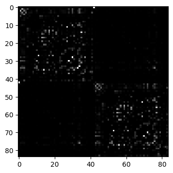
Structural connectivity from the VBI sample

D_loader = vbi.LoadSample(nn=84)
W_empirical = D_loader.get_weights()
n_nodes = W_empirical.shape[0]
print(f"number of nodes: {n_nodes}")

number of nodes: 84

fig, ax = plt.subplots(1, 1, figsize=(4, 4.5))
ax.imshow(W_empirical, cmap="gray", vmin=0, vmax=1);

Base params for inference simulations

params_inf = dict(
    weights=W_empirical,
    dt=0.1,
    t_end=2000.0,
    t_cut=101.0,
    noise_amp=0.001,
    g_e=0.0,
    g_i=0.0,
    P=1.22,
    RECORD_EI="EI",
    decimate=1,
    seed=INFER_SEED,
)

wc_model = WC_sde(params_inf)
print(wc_model)

Wilson-Cowan (Numba) parameters:
nn = 84
dt = 0.1
t_end = 2000.0
t_cut = 101.0
decimate = 1
noise_amp = 0.001
g_e = 0.0
g_i = 0.0
a_e = 1.3
a_i = 2.0
b_e = 4.0
b_i = 3.7
k_e = 0.994
k_i = 0.999

Feature extraction config (spectral stats via Welch)

def preprocess(x):
    """Optional preprocessing hook (here: identity)."""
    # x = x - np.mean(x, axis=1, keepdims=True)
    return x

def simulate_to_features(params_dict: dict, ge_value: float, cfg, return_labels: bool = False):
    """
    Run WC SDE with a given g_e, then extract feature vector for E.
    """
    sde = WC_sde(params_dict)
    sim = sde.run({"g_e": ge_value})
    stat_vec = extract_features(
        [sim["E"].T],
        fs=1.0 / params_dict["dt"] / params_dict["decimate"],
        cfg=cfg,
        preprocess=preprocess,
        preprocess_args={},
        n_workers=1,
        verbose=False,
    )
    values = stat_vec.values  # shape: (1, n_features)
    if return_labels:
        return values[0], stat_vec.labels
    return values[0]

Build a spectral config focused on summary stats

nperseg = 1024
cfg = get_features_by_domain(domain="spectral")
cfg = get_features_by_given_names(cfg, names=["spectrum_stats"])
cfg = update_cfg(
    cfg,
    "spectrum_stats",
    parameters={
        "fs": 1.0 / (params_inf["dt"] * params_inf["decimate"]) * 1000,
        "method": "welch",
        "nperseg": nperseg,
        "average": True,
    },
)
report_cfg(cfg)

Selected features:
------------------
■ Domain: spectral
 ▢ Function:  spectrum_stats
   ▫ description:  Computes the spectrum of the signal.
   ▫ function   :  vbi.feature_extraction.features.spectrum_stats
   ▫ parameters :  {'fs': 10000.0, 'nperseg': 1024, 'indices': None, 'verbose': False, 'average': True, 'method': 'welch', 'features': ['spectral_distance', 'fundamental_frequency', 'max_frequency', 'max_psd', 'median_frequency', 'spectral_centroid', 'spectral_kurtosis', 'spectral_variation']}
   ▫ tag        :  all
   ▫ use        :  yes

Batch simulations → features (with LOAD_DATA switch)

from vbi.utils import BoxUniform
import tqdm

Prior over g_e

N_SIM = 500
g_min, g_max = 0.0, 1.0
prior = BoxUniform(low=[g_min], high=[g_max])
theta = prior.sample((N_SIM,), seed=INFER_SEED).astype(np.float32)  # (N_SIM, 1)

Toggle this to skip recomputation and load saved features instead

LOAD_DATA = True # set to False to regenerate data, load otherwise if available
SIM_DATA_PATH = os.path.join(OUTPUT_DIR, "simulated_data.npz")

def run_batch_features(params_dict: dict, theta_values: np.ndarray, cfg, n_workers: int = -1):
    """
    Parallel feature extraction across theta samples.
    Returns a list of feature vectors.
    """
    def _tick(_):
        pbar.update()
    n = len(theta_values)
    with mp.Pool(processes=n_workers) as pool:
        with tqdm.tqdm(total=n) as pbar:
            async_results = [
                pool.apply_async(
                    simulate_to_features,
                    args=(params_dict, float(theta_values[i]), cfg),
                    callback=_tick,
                )
                for i in range(n)
            ]
            return [r.get() for r in async_results]

Compute or load features

if LOAD_DATA and os.path.exists(SIM_DATA_PATH):
    data = np.load(SIM_DATA_PATH, allow_pickle=True)
    X_features = data["X"]
    theta = data["theta"]
    feature_labels = list(data["labels"])
    print(f"Loaded features from {SIM_DATA_PATH} → X shape {X_features.shape}")
else:
    feature_example, feature_labels = simulate_to_features(params_inf, float(theta[0]), cfg, return_labels=True)
    print(np.array(feature_example).shape)
    print(feature_labels)
    X_list = run_batch_features(params_inf, theta, cfg, n_workers=10)
    X_features = np.array(X_list)
    np.savez(SIM_DATA_PATH, theta=theta, X=X_features, labels=np.array(feature_labels, dtype=object))
    print(f"Saved features to {SIM_DATA_PATH} → X shape {X_features.shape}")

(8,)
['spectral_distance_0', 'fundamental_frequency_0', 'max_frequency_0', 'max_psd_0', 'median_frequency_0', 'spectral_centroid_0', 'spectral_kurtosis_0', 'spectral_variation_0']

100%|██████████| 500/500 [00:36<00:00, 13.77it/s]

Saved features to output/wilson_cowan_sde_numba_cde_/simulated_data.npz → X shape (500, 8)

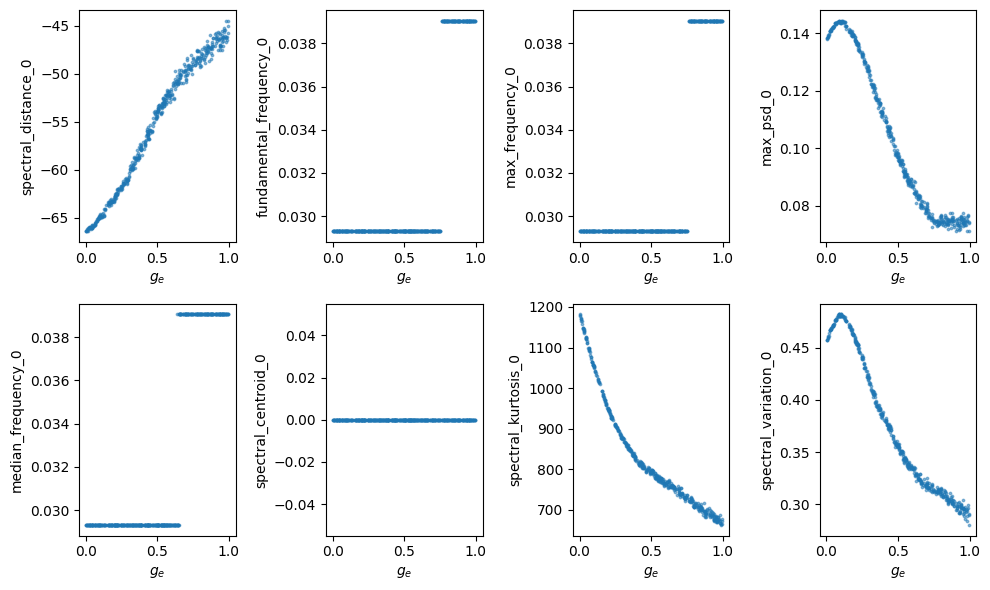
Quick diagnostics: feature vs g_e

fig, axes = plt.subplots(2, 4, figsize=(10, 6))
axes = axes.flatten()
for i in range(min(len(axes), X_features.shape[1])):
    axes[i].scatter(theta, X_features[:, i], s=3, alpha=0.5)
    axes[i].set_xlabel(r"$g_e$")
    axes[i].set_ylabel(feature_labels[i])
plt.tight_layout()

Feature filtering (drop near-constant features)

import pandas as pd

df_features = pd.DataFrame(X_features, columns=feature_labels)
remaining_features = df_features.columns[df_features.var() > 1e-5].tolist()
remaining_idxs = [df_features.columns.get_loc(col) for col in remaining_features]

print("Kept features:", remaining_features)

Kept features: ['spectral_distance_0', 'fundamental_frequency_0', 'max_frequency_0', 'max_psd_0', 'median_frequency_0', 'spectral_kurtosis_0', 'spectral_variation_0']

theta_true = 0.27
x_observed = simulate_to_features(params_inf, theta_true, cfg)[remaining_idxs]

print(x_observed.shape, X_features[:, remaining_idxs].shape)

(7,) (500, 7)

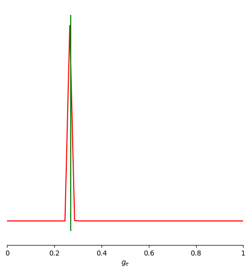
Train MAF estimator and analyze posterior

from vbi.utils import posterior_shrinkage_numpy, posterior_zscore_numpy
import autograd.numpy as anp

rng = anp.random.RandomState(INFER_SEED)
maf = MAFEstimator(n_flows=4, hidden_units=64)

maf.train(
    theta.astype(np.float32),
    X_features[:, remaining_idxs].astype(np.float32),
    n_iter=500,
    learning_rate=2e-4,
)

Inferred dimensions: param_dim=1, feature_dim=7

Training: 100%|██████████| 500/500 [00:10<00:00, 45.61it/s, patience=0/20, train=-2.0224, val=-2.3031]

n_samples = 5000
samples = maf.sample(x_observed, n_samples=n_samples, rng=rng)[0]

shrinkage = posterior_shrinkage_numpy(theta, samples)
zscore = posterior_zscore_numpy(theta_true, samples)

print("True parameters:      ", theta_true)
print("MAF mean estimate:    ", np.mean(samples, axis=0))
print("Posterior shrinkage:  ", np.array2string(shrinkage, precision=3, separator=", "))
print("Posterior z-score:    ", np.array2string(zscore, precision=3, separator=", "))

True parameters:       0.27
MAF mean estimate:     [0.26878434]
Posterior shrinkage:   [1.]
Posterior z-score:     [0.276]

from vbi.plot import pairplot_numpy

limits = [(g_min, g_max)]
points = np.array(theta_true).reshape(1, -1)

fig, ax = pairplot_numpy(
    samples=samples,
    limits=limits,
    points=points,
    figsize=(8, 6),
    labels=[r"$g_e$"],
    diag="kde",
    fig_kwargs=dict(
        points_offdiag=dict(marker="*", markersize=5),
        points_colors=["g"],
    ),
    diag_kwargs={"mpl_kwargs": {"color": "r"}},
    upper_kwargs={"mpl_kwargs": {"cmap": "Blues"}},
)